Overview

This is a CS184 Project. This time, it’s just the bare minimum rubric items because I’m a little swamped by work. You can still find pretty images peppered within the post though, if those interest you : )

In this project, I implemented a ray generation routine that starts with input coordinates from the image space and generates a ray with coordinates in the world space. I also implemented the ray-intersection routines for two types of primitives: spheres and triangles. Then, I implemented both direct and indirect lighting to achieve global illumination. Finally, I implemented an adaptive sampling feature so the program can intelligently decide when to stop sampling.

Rubric

Part 1

Walk through the ray generation and primitive intersection parts of the rendering pipeline.

Ray Generation

Initially, the pixel position we need to render comes in the form of $(x, y)$ that’s in image space, i.e. it indicates which pixel is being rendered. We first add a random offset to this coordinate to determine which point in the square encompassed by $(x,y)$ and $(x + 1, y + 1)$ we will sample. Then, we divide the result by vector $(w, h)$ to obtain the normalized coordinates.
To generate a ray, we start with defining the two corners: the bottom left and the upper right in camera space. Since the x and y positions are now mapped to the range $[0, 1)$ , we can simply do a linear interpolation of the corner points using those two parameters:

1
2
3

// Element-wise vector arithmetic
Vector3D v = bottomLeft + Vector3D(x, y) * (upperRight - bottomLeft);
normalize(v);

The ray we generate originates from the camera origin and has a direction of v. Both vectors are converted from camera space to world space using the c2w matrix.
Finally, we set max_t and min_t of the ray to limit the minimum and maximum rendering distance.
Minor implementation note: Since c2w does not use homogenous coordinates, we have to manually add the position of the camera to the origin to obtain the origin of the ray. We don’t have to do this for v because v itself is a delta.

Now that we have our ray, it’s time to find out where it intersects with the scene so we can use it to calculate light transport.

Primitive Intersection with Spheres

Sphere intersection is relatively straight-forward, not least because spheres can be expressed by the simple equation, where $\mathbf{c}$ is the center of the sphere and $R$ is the radius of the sphere.

|(\mathbf{p} - \mathbf{c})|^2 = R^2

Given that a ray can be expressed as

\mathbf{r}(t) = \mathbf{o} + t \mathbf{d}

We can set $\mathbf{p} = \mathbf{r}(t)$ to obtain

|(\mathbf{o} + t \mathbf{d} - \mathbf{c})|^2 = R^2

This is just a quadratic equation, meaning that we can use the quadrtic equation formula to solve for $t$ . If we get two solutions, then then the ray must first enters the sphere and then exists it. If we get one solution, then the ray is tangent to the sphere. If we get no real solutions, then the ray misses the sphere.

Primitive Intersection with Triangles

For triangle intersection, I simply implemented the Moller Trumbore Algorithm:

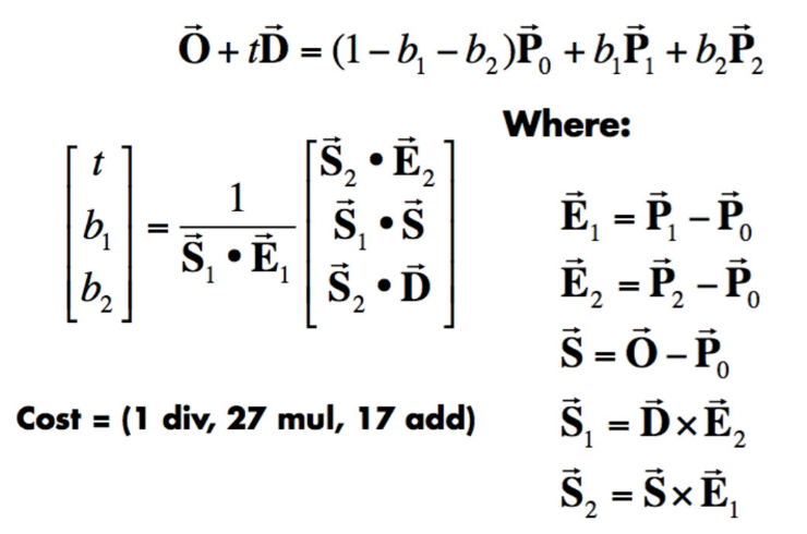
What’s nice about this algorithm is that aside from being fast, it also returns the barycentric coordinates at the intersection, which can be used to determine the normal vector by interpolating the three vertex normal vectors.

For both intersection routines (sphere and triangle), all $t$ values outside of the [min_t, max_t] range are ignored. Furthermore, once we find a valid intersection, we update max_t so that only closer intersection points are considered. Finally, if we end up with a valid intersection, we update the fields of the isect object with useful information, such as the value of the final t, the bsdf, the normal vector, and the Primitive object that this ray intersected with.

Explain the triangle intersection algorithm you implemented in your own words.
To see how we can derive the Moller Trumbore Algorithm, we can start with defining the unknowns: $t$ and the barycentric coordinates $(b_0, b_1, b_2)$ . Since $b_0 + b_1 + b_2 = 1$ , we really only have three unknowns $t$ , $b_1$ , and $b_2$ .

Then we use a similar approach to how we derived the intersection formula for spheres: substituting a point on the triangle $\mathbf{P}$ with a point on the ray’s path.

\mathbf{O} + t\mathbf{D} = (1 - b_1 - b_2)\mathbf{P_0} + b_1\mathbf{P_1} + b_2\mathbf{P_1}

Moving the unknowns to a single vector, we obtain the equation

\begin{bmatrix} -\mathbf{D} & (\mathbf{P_1} - \mathbf{P_0}) & (\mathbf{P_2} - \mathbf{P_1}) \end{bmatrix} \begin{bmatrix}t \\ b_1 \\ b_2 \end{bmatrix} = (\mathbf{O} - \mathbf{P_0})

Taking the inverse of the left matrix and multiplying it on both sides, we obtain an equation that we can use to directly calculate the values of our unknowns. However, to reach the simplicity of the Moller Trumbore Algorithm, we also need to transform our answer using Cramer’s Rule and an equation that links the determinant of a 3x3 matrix to the cross products of its column vectors $|\mathbf{A, B, C}| = -(\mathbf{A} \times \mathbf{C}) \cdot \mathbf{B} = -(\mathbf{C} \times \mathbf{B}) \cdot \mathbf{A} = -(\mathbf{B} \times \mathbf{A}) \cdot \mathbf{C}$ . Here, I omit the actual derivation, but with those two equations the procedure is fairly mechanical.

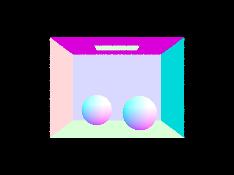
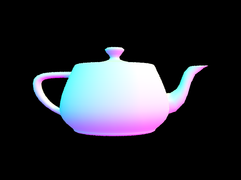
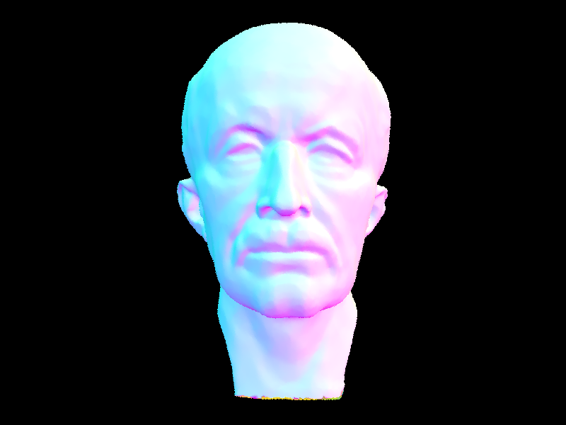
Show images with normal shading for a few small .dae files.

Part 2

Walk through your BVH construction algorithm. Explain the heuristic you chose for picking the splitting point.

We first loop over all the primitives and use them to expand a bounding box. This bounding box is thus the bounding box of the current node. Then, we check if the number of primitives is smaller than max_leaf_size. If it is, then we can return the node.

Otherwise, we proceed to find the variance of the centroid of the bounding boxes of every primitive object passed in on each axis. We take the axis that has the largest variance as the axis that we will split with.

We sort the primitives in place using a custom comparator that compares the location of the primitives on the selected axis. Then, we take the middle element of the primitives as a splitting point and pass each half to recursive calls of construct_bvh. Finally, we assign the returned nodes as children.

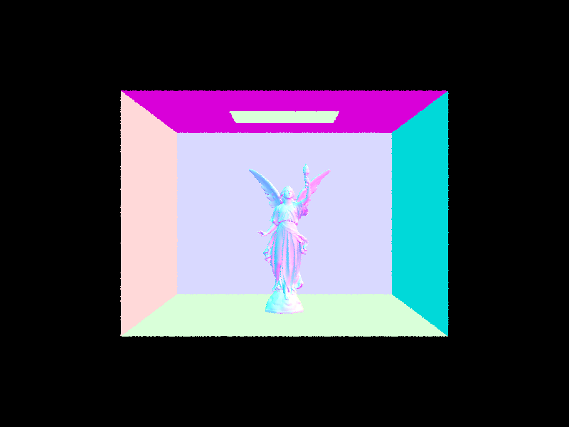
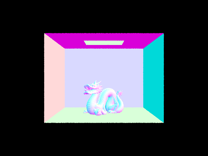
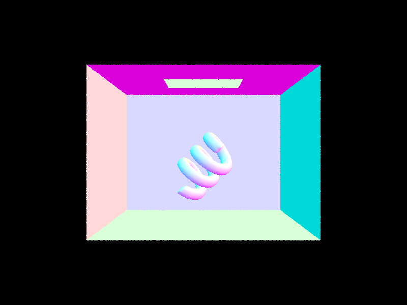
Show images with normal shading for a few large .dae files that you can only render with BVH acceleration.

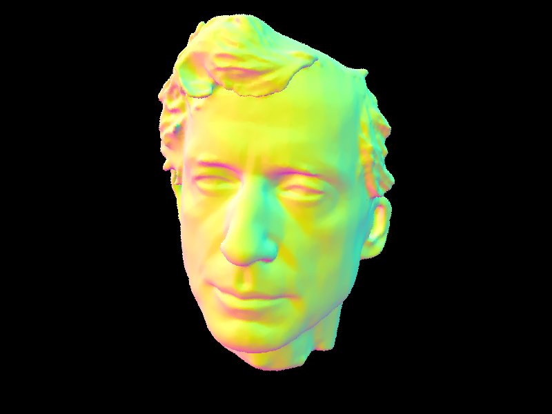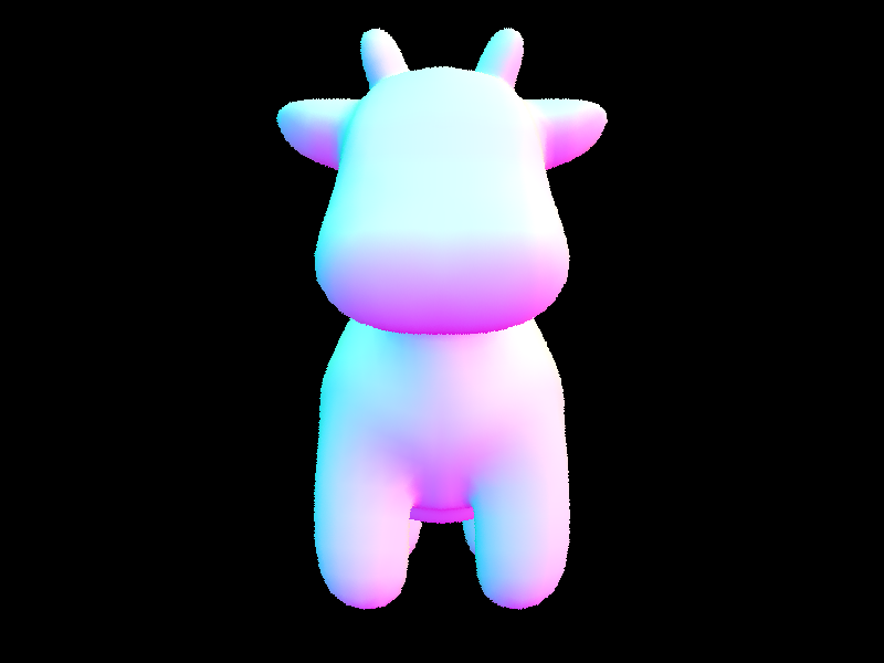
Compare rendering times on a few scenes with moderately complex geometries with and without BVH acceleration. Present your results in a one-paragraph analysis.
The coil scene takes 74 seconds to render on a 12-core machine without bvh, but only takes 0.0301 seconds with BVH. The cow scene takes 50 seconds without bvh, but only takes 0.0296 seconds using bvh. This drastic improvement can be explained by the fact that a well-constructed bvh allows the ray to selectively test against a subset of the scene that it passes through instead of testing against every primitive. At each step of the BVH traversal, if the ray does not intersect the bounding the box of the current node, the whole node is ignored, bringing the runtime down from $O(n)$ to $O(log(n))$ in the ideal amortized case.

Part 3

Walk through both implementations of the direct lighting function.

Uniform Random Sampling

In estimate_direct_lighting_hemisphere, we first make a local coordinate system for the hit point, with the normal pointing in the z-direction. Furthermore, w_out (the direction that the outgoing light takes) can be obtained directly from inverting the direction of the ray. The point that the ray is hitting can be obtained by r.o + r.d * isect.t.

Then, we loop through the number of samples requested, each time creating a new random w_in (the direction that the incoming light hits this surface) using hemisphereSampler->get_sample(). We create a new ray using hit_p as the origin and w_in as the direction. We need to make sure that both are in world coordianates, because we will use this ray to test intersection with the scene. Also, caution was made to offset the origin of the ray by EPS_F to circumvent numerical precision errors.

Next, we test this ray against the scene to see if we hit a light. If we do, we add the contribution to our answer using the equation 2 * PI * light_i.bsdf->get_emission() * dot(isect.n, w_in) * isect.bsdf->f(w_out, w_in). The first term is the inverse pdf, the second term is the emission from the light, the third term comes from Lambert’s cosine law, and the fourth term is the BSDF of the current point.

Once the loop finishes, we divide the answer by the number of samples taken and return it.

Importance Sampling

The procedure is largely the same as the uniform random sampling function. The key differences are:

We loop through each light and attempt to shoot shadow rays towards it.
If the light is a point source, then only one sample is taken. If the light is an area light, then we tell the light to pick an angle using light->sample_L and repeat the process ns_area_light times.
We need to check if the normal of the surface and the direction sampled by the light match. If they don’t, the radiance is automatically 0.
Instead of dividing the total number of samples in the end, we divide by the number of samples per light when we are in the loop. For example, for point sources, we divide by 1. For area lights, we divide by ns_area_light. This measure keeps the estimator unbiased.

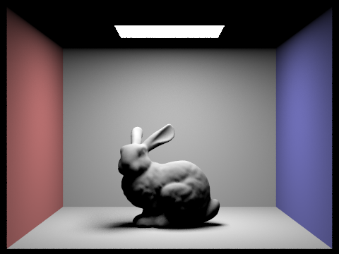
Show some images rendered with both implementations of the direct lighting function.
All of the images below are rendered using 32 samples per pixels and 32 light rays.
Command: -t 12 -s 32 -l 32 -m 6 -r 480 360


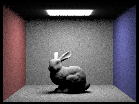Uniform Random	Importance Sampling

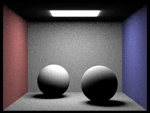
Focus on one particular scene with at least one area light and compare the noise levels in soft shadows when rendering with 1, 4, 16, and 64 light rays (the -l flag) and with 1 sample per pixel (the -s flag) using light sampling, not uniform hemisphere sampling.

1 light ray(s)	4 light ray(s)

16 light ray(s)	64 light ray(s)

As we can observe, when we increase the number of light rays per sample the noise level in soft shadows decreases. This is because by generating more light rays and averaging the results we are obtaining a better estimate of the actual amount of the light that is at one spot through our unbiased estimator.

Part 4

Walk through your implementation of the indirect lighting function.

In est_radiance_global_illumination, we first check if the depth of the ray is not zero. If so, we proceed to generate direct and indirect lighting. If not, we only return zero_bounce_radiance.

Inside at_least_one_bounce_radiance is where global illumination happens. First, ray depth is checked as a base case. If we reach 0, a black Spectrum is returned. Next, direct illumination is calculated via calling one_bounce_radiance. (Notice that although we call this direct illumination, if we are not in the first recursive call, then this result will contribute to the indirect illumination of a prior call). Then, we create a new ray in the direction of bsdf->sample_f. We test intersection using that ray with the scene. If it doesn’t intersect anything, we are safe to return just the direct illumination. If it does, we perform a coin flip with probability 0.7 to decide whether to continue. In the case we want to continue, we recursively call at_least_one_bounce_radiance and add the (scaled) result to the output. Here that this result is scaled by 1) the BSDF of the current surface 2) Lamberts’ Cosine Law 3) inverse of the Russian Roulette probability 4) inverse of the pdf returned by bsdf->sample_f.

This concludes the implementation of indirect illumination.

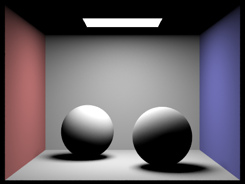
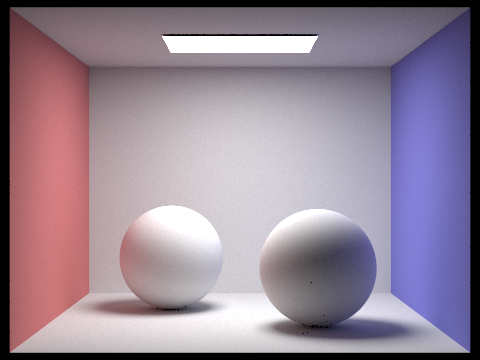
Show some images rendered with global (direct and indirect) illumination. Use 1024 samples per pixel.

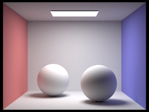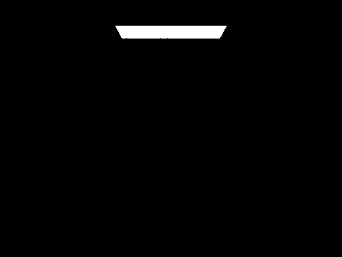
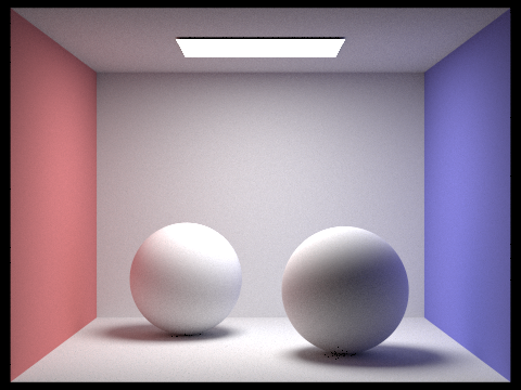
Pick one scene and compare rendered views first with only direct illumination, then only indirect illumination. Use 1024 samples per pixel.

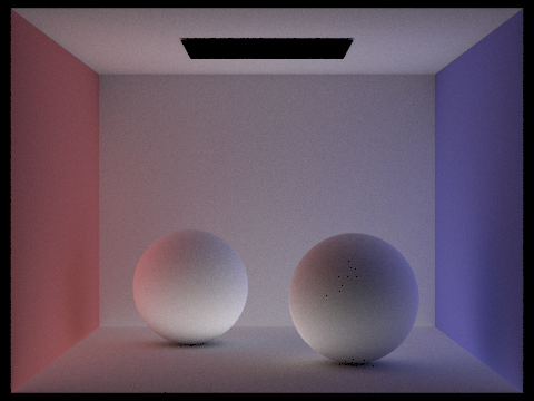Notice that surfaces only show their original color with direct lighting, but show the colors reflected from neighboring surfaces with indirect lighting.

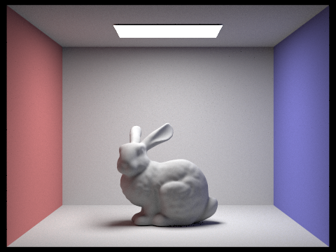
For CBbunny.dae, compare rendered views with max_ray_depth set to 0, 1, 2, 3, and 100 (the -m flag). Use 1024 samples per pixel.

Max ray depth: 0	Max ray depth: 1
Max ray depth: 2	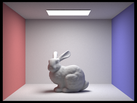Max ray depth: 3

Max ray depth: 100

Increasing max_ray_depth seems to give us diminishing returns. This makes sense, because when the light bounces farther its contribution to the final radiance is going to diminish with the cosine term at every bounce. As we go from 0 to 3, the scene becomes visibly brighter and more vibrant. However, the difference between a max_ray_depth of 3 and 100 does not seem very significant, though still noticeable. In particular, the blue/red tint is more pronounced on the white walls when we increase max_ray_depth to 100.

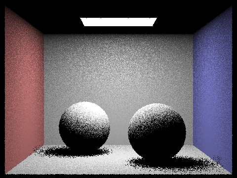
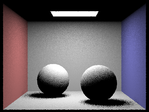
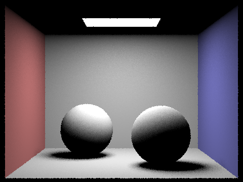
Pick one scene and compare rendered views with various sample-per-pixel rates, including at least 1, 2, 4, 8, 16, 64, and 1024. Use 4 light rays.

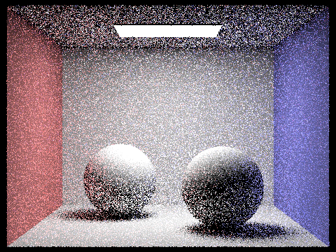Samples per pixel: 1	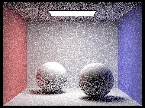Samples per pixel: 2
Samples per pixel: 4	Samples per pixel: 8
Samples per pixel: 16	Samples per pixel: 64

Samples per pixel: 1024

As we may expect, when we increase the sample rate per pixel, the noise goes down.

Part 5

Walk through your implementation of the adaptive sampling.
In raytrace_pixel, we create two new variables s0 and s1 which tracks the sum of the illuminance and illuminace^2 so far. In every iteration of the loop, we check if the number of samples performed is divisible by samplesPerBatch. If it is, we calculate a confidence interval using the formula provided in the spec and compare it with maxTolerance * mu. If we reach the desired tolerance, we write the current number of samples to the sample_rate buffer and exit the loop.
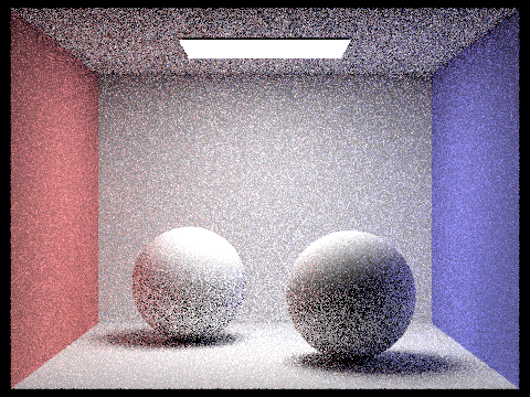
Pick one scene and render it with at least 2048 samples per pixel. Show a good sampling rate image with clearly visible differences in sampling rate over various regions and pixels. Include both your sample rate image, which shows your how your adaptive sampling changes depending on which part of the image you are rendering, and your noise-free rendered result. Use 1 sample per light and at least 5 for max ray depth.

Output	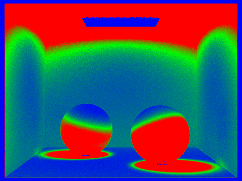Sample rate

Command: ./pathtracer -t 12 -s 2048 -l 1 -m 5 -f CBspheres_2048_1_GI.png -r 480 360 ../dae/sky/CBspheres_lambertian.dae

Markz's Blog

Path-Tracing