This is a CS184 Project. For graders, if you are looking for a list of rubric items and their locations within this post, please scroll to the bottom of the page. For everyone else, please read on.

Overview

In this post, we are going to talk about Bezier Curves and the Half Edge Data Structure. Technically, those two are completely distinct topics that should belong to two posts, but CS184 made them into one project, so here we are.

Bezier curves are widely used in programs like PhotoShop to draw smooth curves. It is the default curve type for the pen tool in PhotoShop. In this post, we’ll explore how Bezier curves can be generated programmatically using the de Casteljau method. We’ll also briefly explore the 2D generalization of Bezier curves - Bezier surfaces.

The half edge data structure is one way to represent 3D meshes that are composed of triangles. It is powerful because it allows operations such as neighbor lookup in O(n) time, where n is the number of neighbors of a vertex, edge, or face. In a naive data structure where simply store a list of triangles, the same operation takes O(N), where N is the total number of triangles.

Bezier Curves and the de Casteljau method

A Bezier Curve is defined by two or more control points. A Bezier curve of degree n is defined by (n+1) control points. The typical Bezier curve we see in various graphic processing programs is of degree 3, because it is relatively easy to predict how the curve would change once we manipulate the control points and is also very expressive. The first and the last control points define where the curve start and end, and all the control points contribute to the curvature of the curve. For example, here’s a curve I drew in PhotoShop (it is of degree 3):

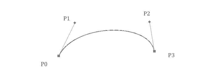
Unfortunately there's some very apparent aliasing

The de Casteljau method provides a way for us to draw any Bezier curve given its control points. It takes in a curve and a single parameter $t$ that is in the range of $[0, 1]$ . It then recursively performs linear interpolations until the curve collapses to a single point, and this point is guaranteed to be on the Bezier curve. All we have to do, therefore, is iterate through $t$ and connect the points outputted by the algorithm.

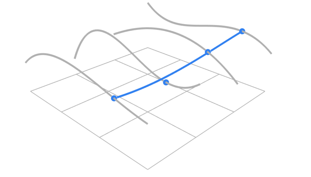
More concretely, the de Casteljau method linearly interpolates between every pair of two adjacent control points (parameterized by $t$ ). Since there are only $(n - 1)$ such pairs if we start with $n$ points, we have decreased our problem size by $1$ . Rinse and repeat until we only have $1$ point left. Here’s a nice diagram that I took and modified from the cs184 course website demonstrating this process for a single $t$ .

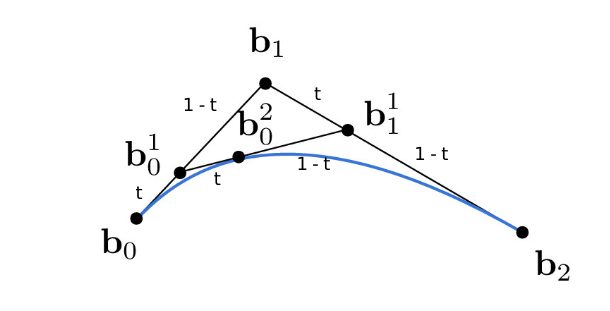
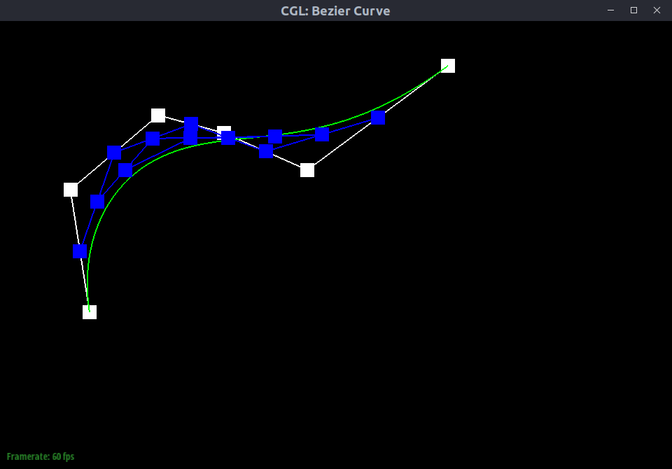
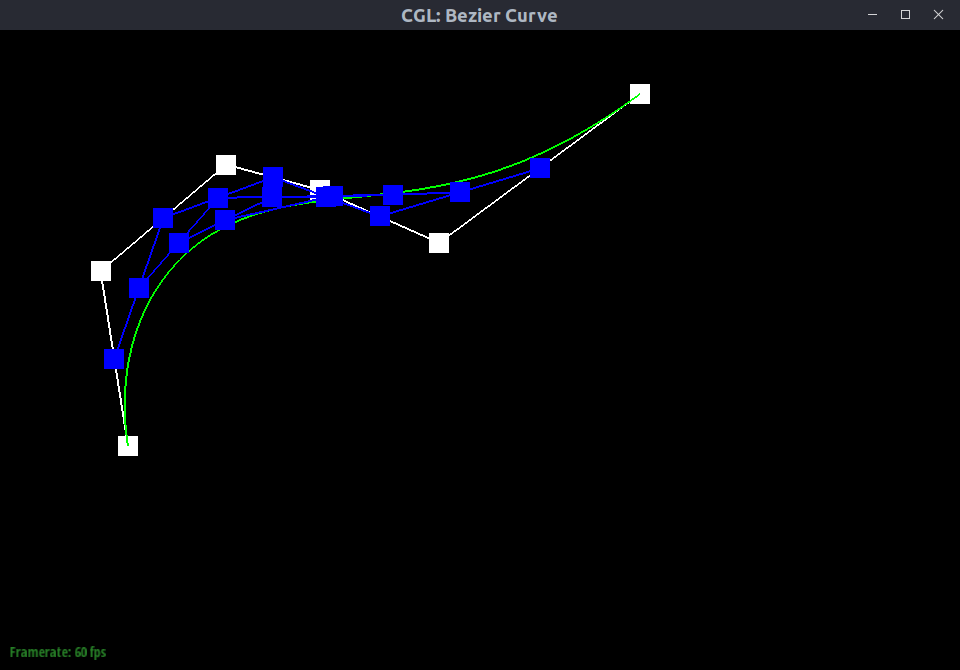
Once we repeat the process for enough $t$ values in the range of $[0, 1]$ , we get the blue line shown above.

Bezier Surfaces

The following explanation borrows some nice visuals from Steven Wittens’s talk Making things with Maths. I recommend checking out his talk too because his slide deck is interactive!

The idea of linearly interpolating control points to obtain a curve generalizes from 1D curves to 3D surfaces too. Before we dive into what that means, let’s first define a function evaluate1D that performs the 1D de Casteljau method described in the above section at parameter t.

1	Vector3D evaluate1D(std::vector<Vector3D> const &points, double t) const;

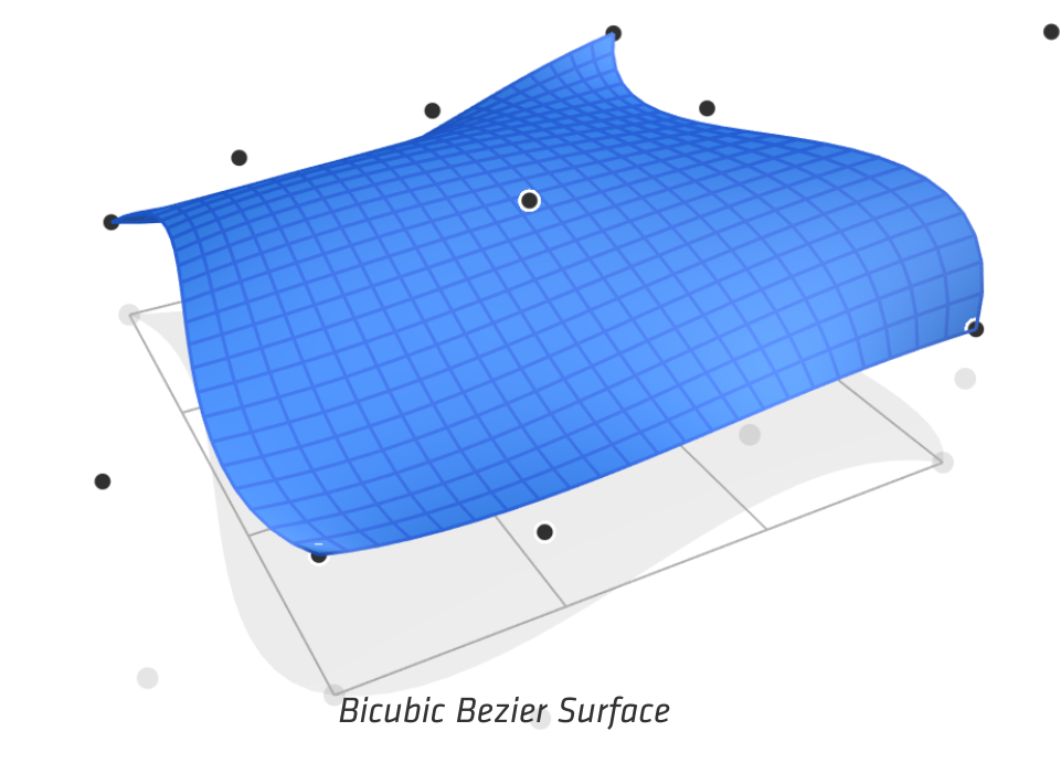
We start with a grid of 4x4 points, though like in the 1D case, we can generalize Bezier surfaces to an arbitrary number of points. We then interpolate each row of 4 points to obtain 4 Bezier curves using evaluate1D.

Image credit goes to Steven

If we parametrized those curves using a variable u, then by setting u to a certain value, we obtain four new control points, each one on a different Bezier curve.

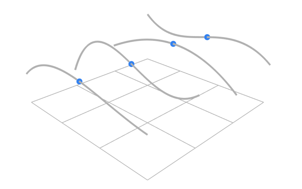
Finally, we apply evaluate1D again to those four points to obtain another Bezier curve. This time will need to pick another variable to parameterize it, e.g. v.

If we sweep this Bezier curve through space by varying u from 0 to 1. We’ll obtain a surface! In the actual implementation, we can obtain every point defined by this 4x4 grid by providing a unique u and v. Below is the pseudocode for doing that.

Vector3D evaluate2D(std::vector<std::vector<Vector3D>> grid, 
                    double u, double v)
{
  std::vector<Vector3D> col;
  for row in grid
    col.push_back(evaluate1D(row, u));
  return evaluate1D(col, v);
}

Half Edge Data Structure

(To be Continued)
I ran out of time so I only wrote the parts included in the rubric. If you are a grader, the items can be found below.

Rubric

Task 1

Briefly explain de Casteljau’s algorithm and how you implemented it in order to evaluate Bezier curves.
For the explanation, see Bezier Curves and the de Casteljau method
As for the actual implementation, I simply looped over the points, multiplied each adjacent pair by the right linear factor, and saved them in another std::vector<Vector2D>.
Take a look at the provided .bzc files and create your own Bezier curve with 6 control points of your choosing. Use this Bezier curve for your screenshots below.
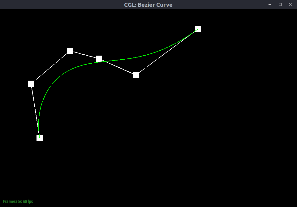
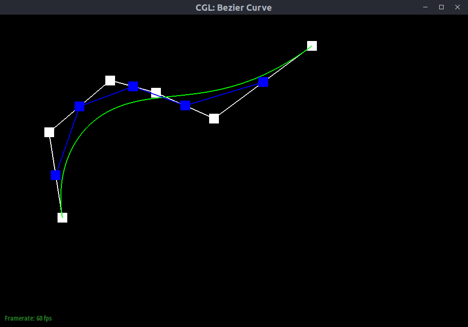
Show screenshots of each step / level of the evaluation from the original control points down to the final evaluated point. Press E to step through. Toggle C to show the completed Bezier curve as well.

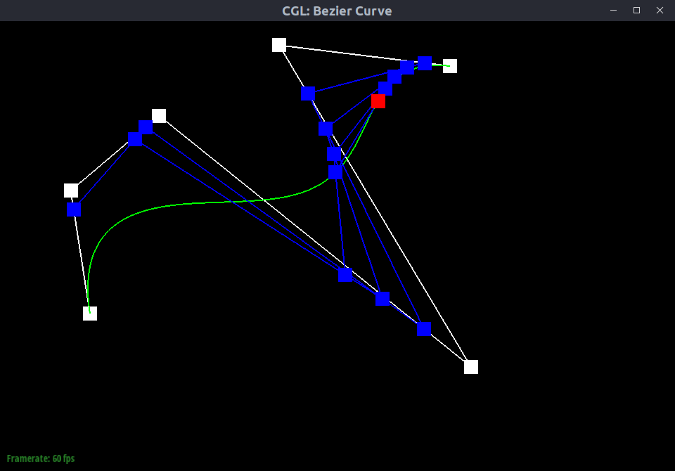
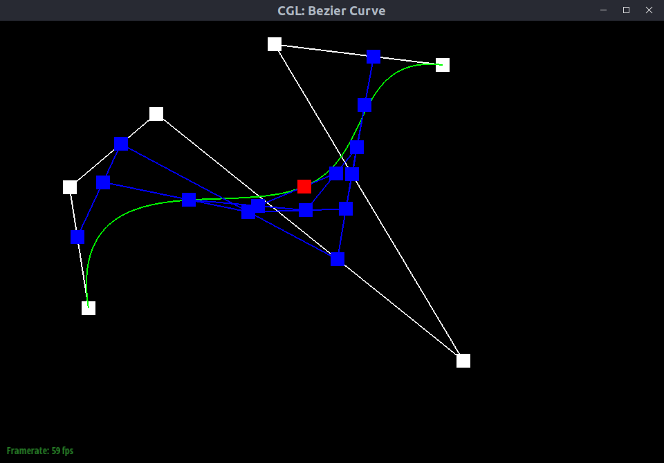
Show a screenshot of a slightly different Bezier curve by moving the original control points around and modifying the parameter tt via mouse scrolling.

Task 2

Briefly explain how de Casteljau algorithm extends to Bezier surfaces and how you implemented it in order to evaluate Bezier surfaces.
See Bezier Surfaces
Show a screenshot of bez/teapot.bez (not .dae) evaluated by your implementation.

Part 3

Briefly explain how you implemented the area-weighted vertex normals.
I first initialize a zero vector as the answer vector. Then, I loop over every edge adjacent to the given vertex by h->twin()->next(). In each iteration, I calculated two vectors that correspond to the two edges of the triangle adjacent to our vertex. By taking their cross product, we obtain a vector normal to the plane of the triangle with a size that’s equal to the area of the triangle. Therefore, we can simply add it to the answer vector. After all iterations, we normalize the answer vector and return it.
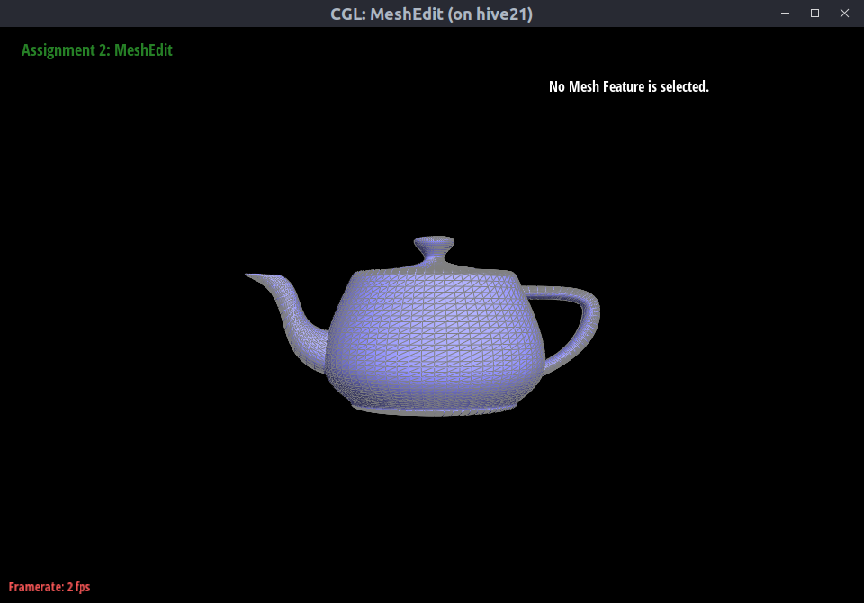
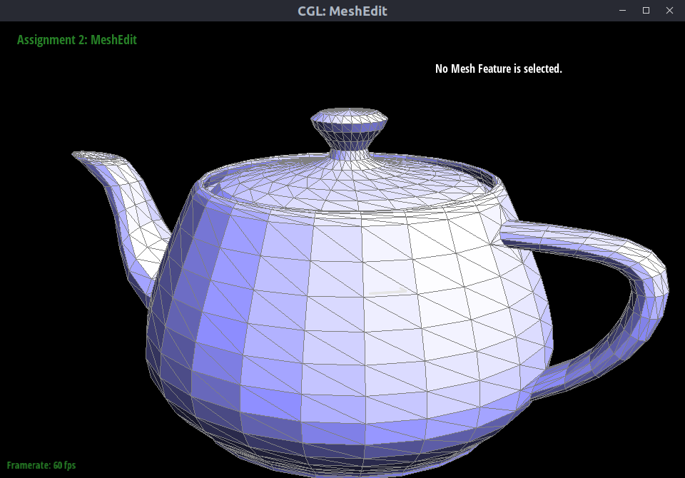
Show screenshots of dae/teapot.dae (not .bez) comparing teapot shading with and without vertex normals. Use Q to toggle default flat shading and Phong shading.

Flat shading, wireframes	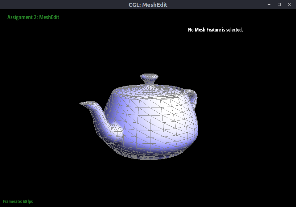Phong shading, wireframes
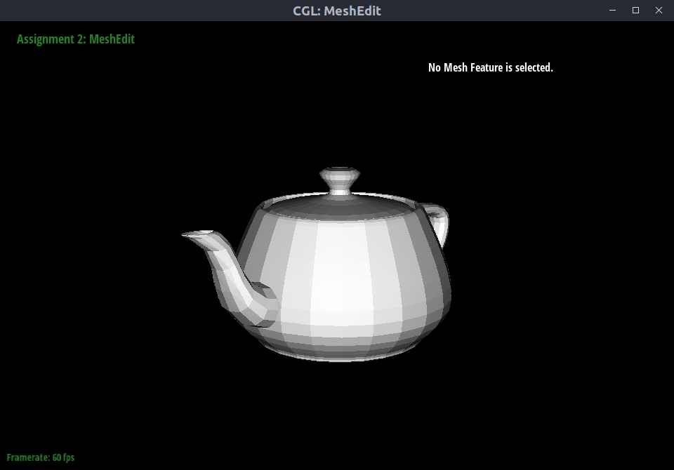Flat shading, no wireframes	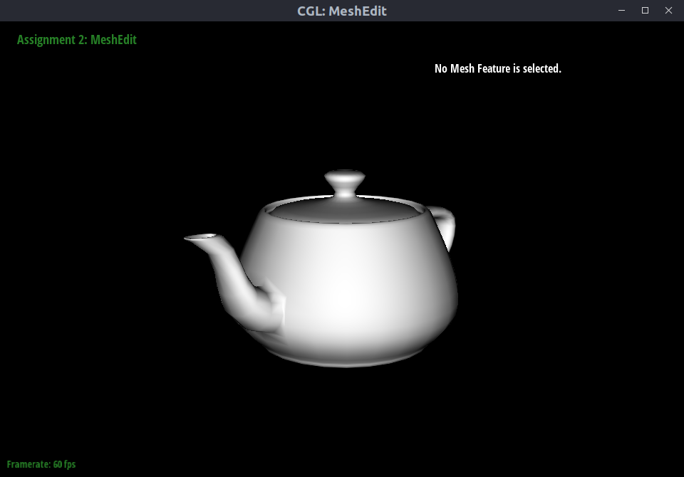Phong shading, no wireframes

Part 4

Briefly explain how you implemented the edge flip operation and describe any interesting implementation / debugging tricks you have used.
I first checked if the edge is on the boundary. If it is, the functions returns immediately. Then, I assigned the relevant edges, faces, and vertices into numbered variables. Finally, I updated the relationships between those variables via pointer assignment.
One interesting implementation trick I used was drawing a diagram on paper first and then assigning variables based on that.
Show screenshots of a mesh before and after some edge flips.

Before flips	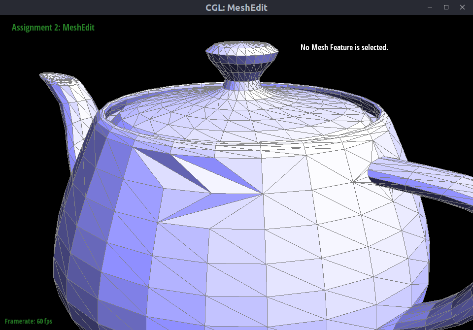After flips

Write about your eventful debugging journey, if you have experienced one.
I did not experience an eventful debugging journey.

Part 5

Briefly explain how you implemented the edge split operation and describe any interesting implementation / debugging tricks you have used.
The procedure is similar to flip, with the exception that there are now memory allocations.
I first checked if the edge is on the boundary. If it is, the functions returns immediately.
Then, I assigned the relevant edges, faces, and vertices into numbered variables. I also allocated 2 new vertices, 3 new edges, 6 new half-edges, and 2 new faces. Finally, I updated the relationships between those variables via pointer assignment.
One interesting implementation trick I used was drawing a diagram on paper first and then assigning variables based on that.
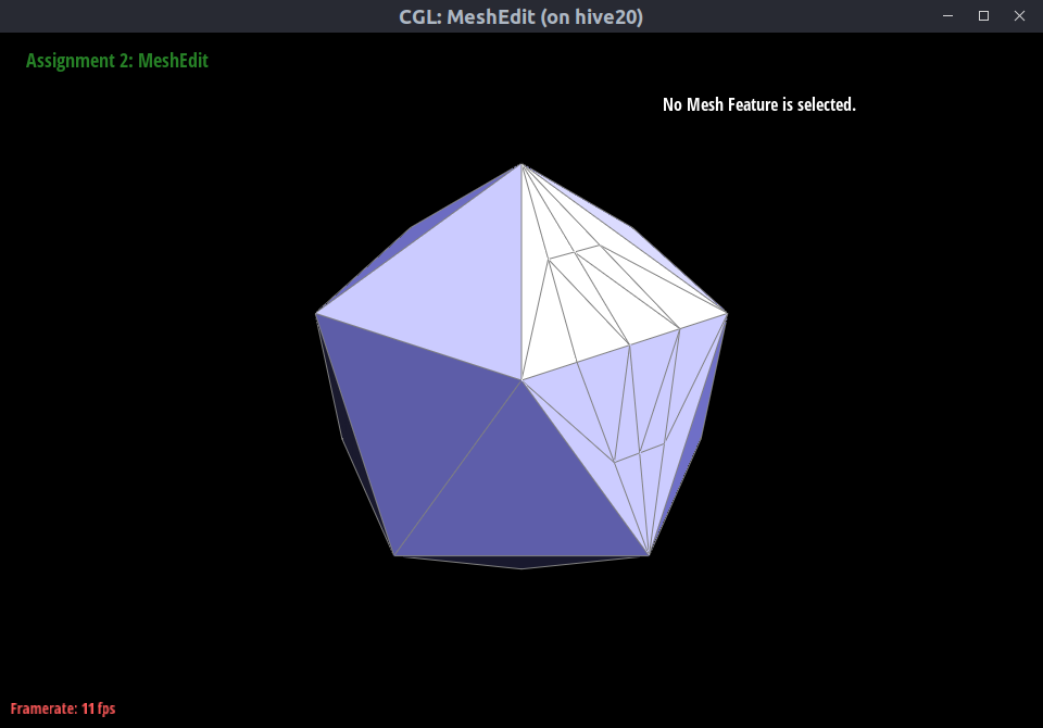
Show screenshots of a mesh before and after some edge splits.

Before splits	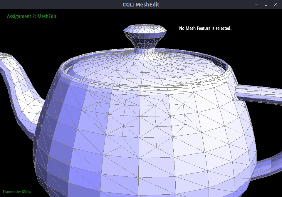After splits

Show screenshots of a mesh before and after a combination of both edge splits and edge flips.

Before splits & flips	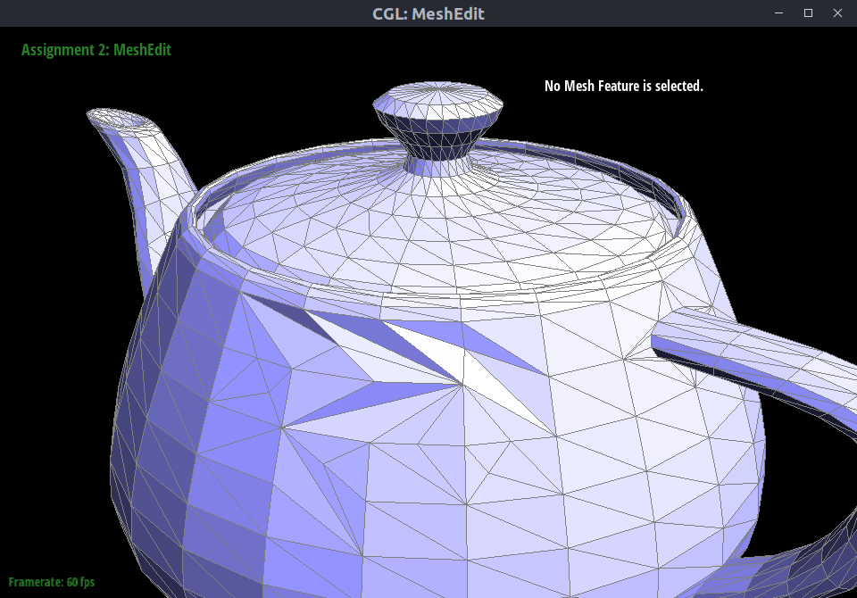After splits & flips

Write about your eventful debugging journey, if you have experienced one.
I did not experience an eventful debugging journey.

Part 6

Briefly explain how you implemented the loop subdivision and describe any interesting implementation / debugging tricks you have used.
I first iterated through all the vertices using the verticesBeginand verticesEnd iterators, during which I marked every vertex as not new, computed the centroid, and stored the new positions.
Then, I iterated through all the edges using edgesBegin and edgesEnd, during which I calculated the new positions of the soon-to-be-added vertices and stored all the existing edges into an std::vector.
I then looped over the old edges again, this time splitting them, updating the newPosition field of the newly added vertices using the value calculated in the previous step, and marking all the newly created edges as new.
As the second to last step, I looped over all the halfedges while selectively flipping new edges that connect to one new and one old vertex.
Finally, I looped over all the vertices and updated their positions to be newPosition.
One debugging trick I used was to only perform portions of the Loop subdivision algorithm and using the visualizer to verify that my results so far are correct. This verification includes walking through the mesh using keyboard shortcuts to ensure the mesh is not malformed and observing the updated positions to see if they seem correct.
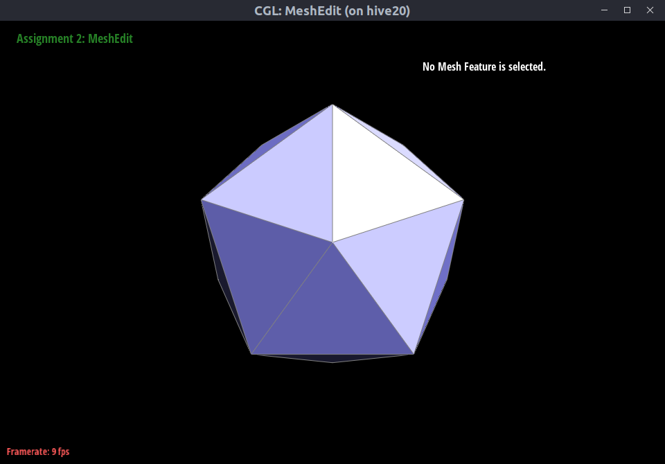
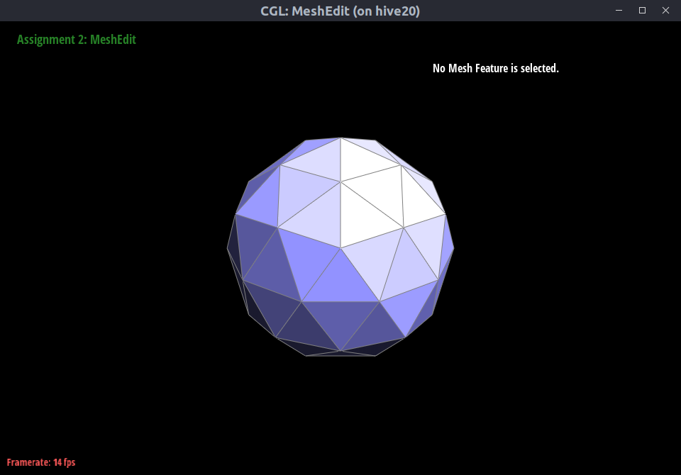
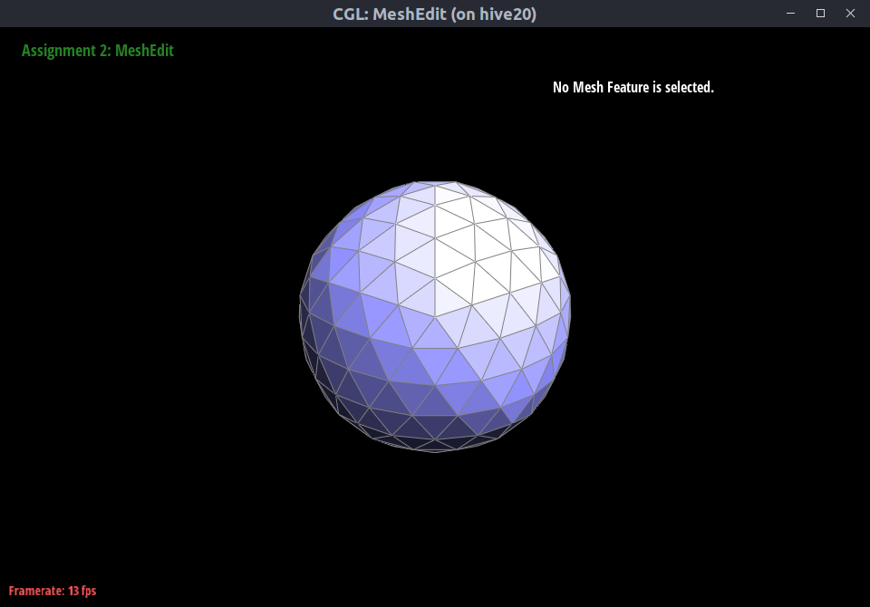
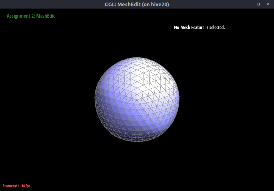
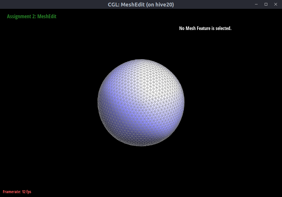
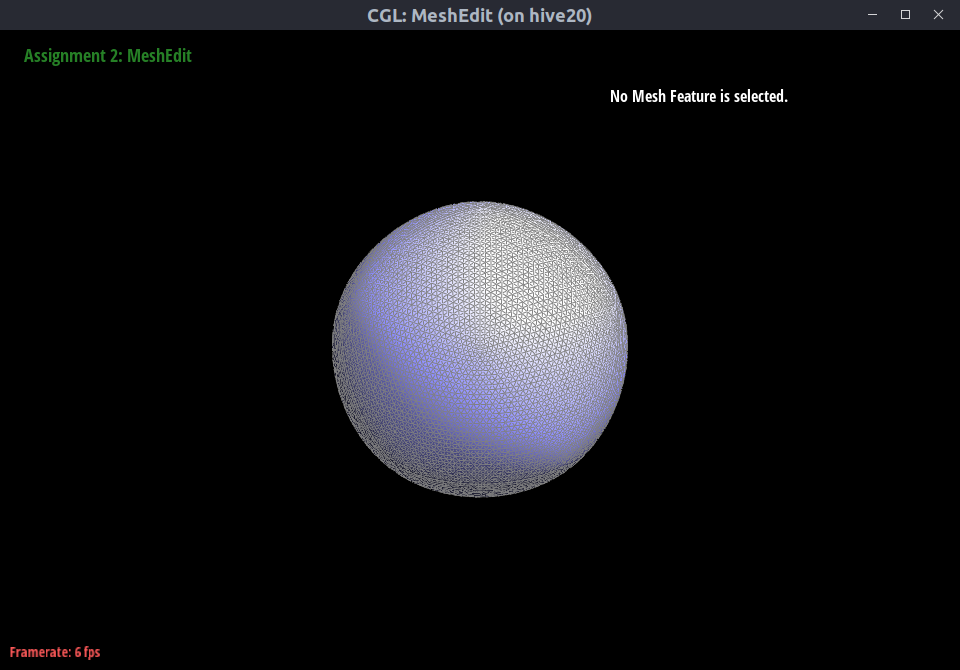
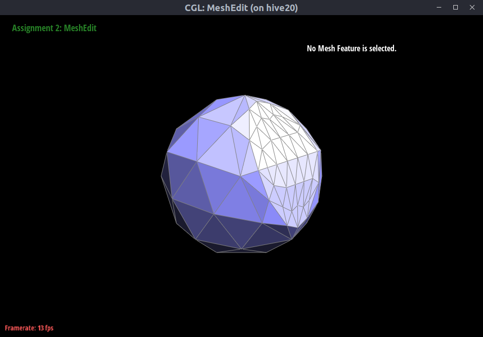
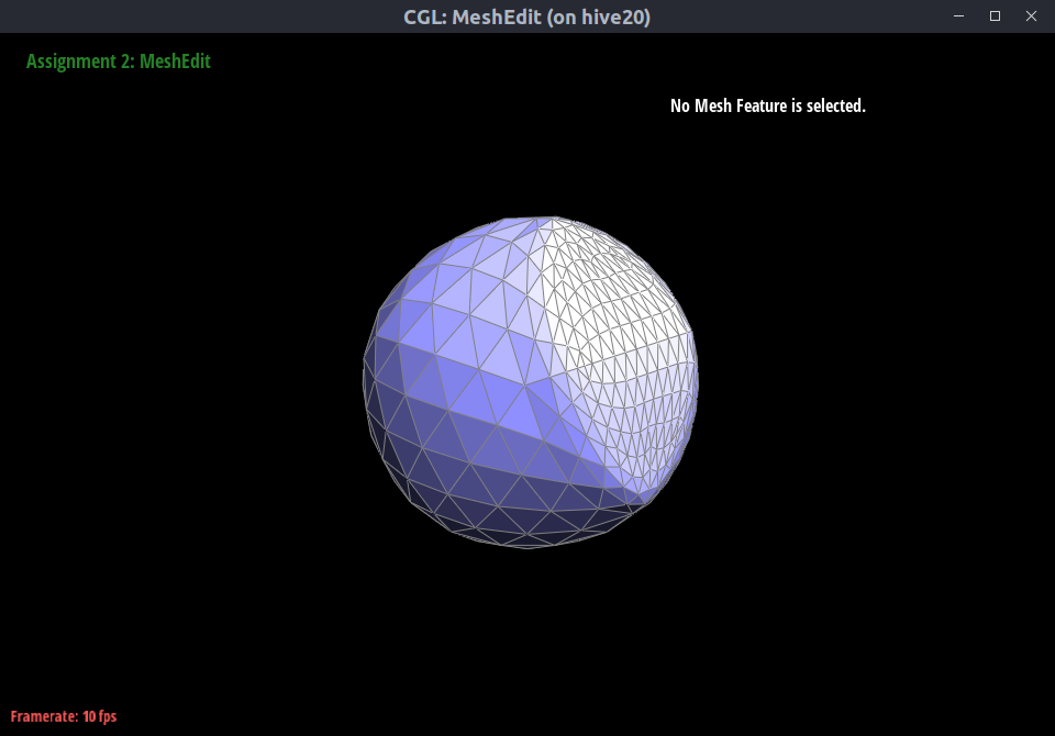
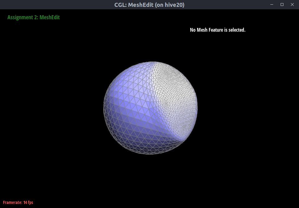
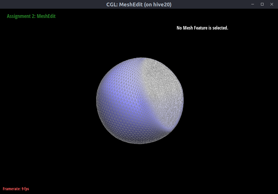
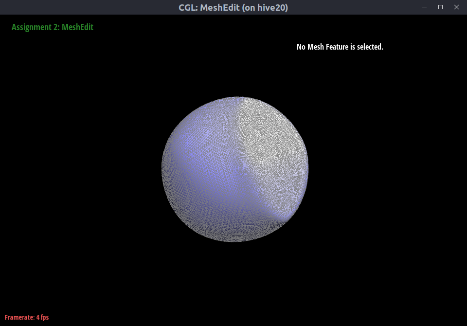
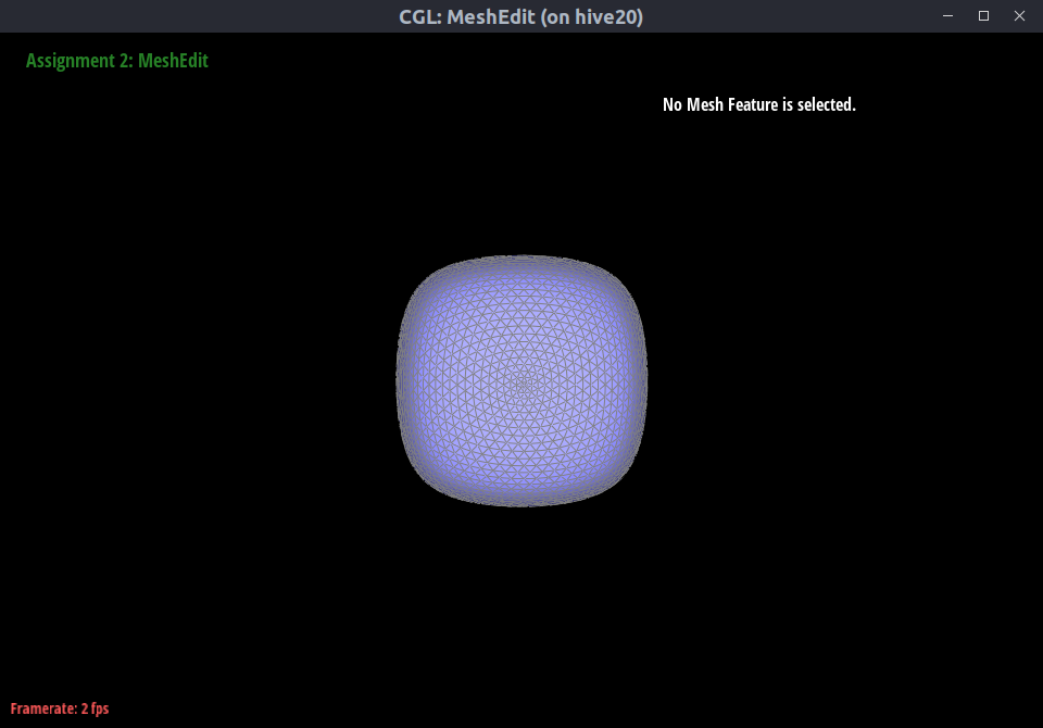
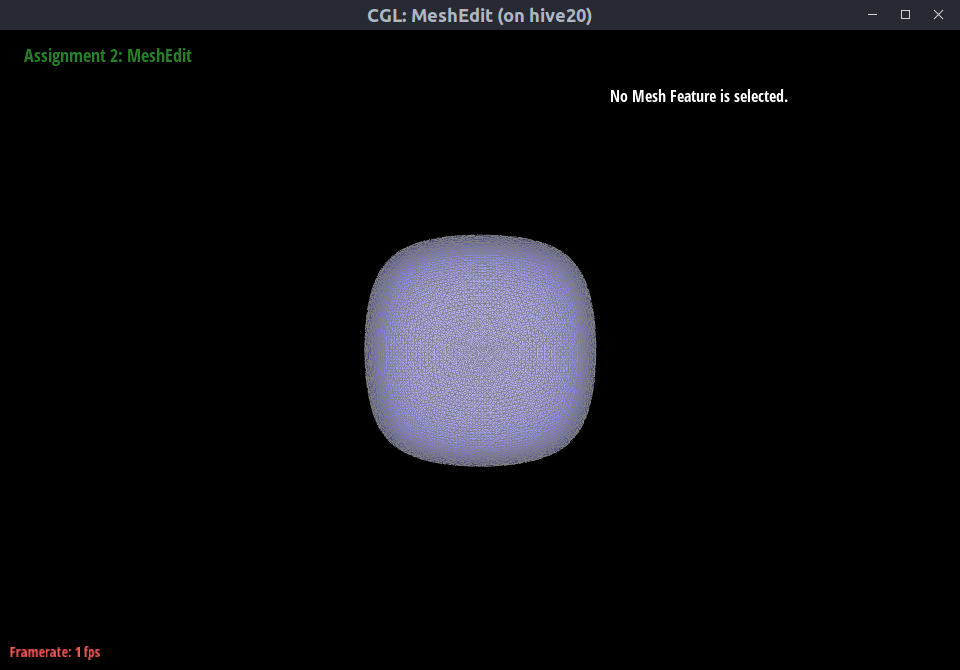
Take some notes, as well as some screenshots, of your observations on how meshes behave after loop subdivision. What happens to sharp corners and edges? Can you reduce this effect by pre-splitting some edges?
The sharp corners and edges become smoother. As we can observe below.

However, if we pre-split the edges on the face adjacent to the edge we want preserve, we can palliate the effect of Loop subdivision on that edge.

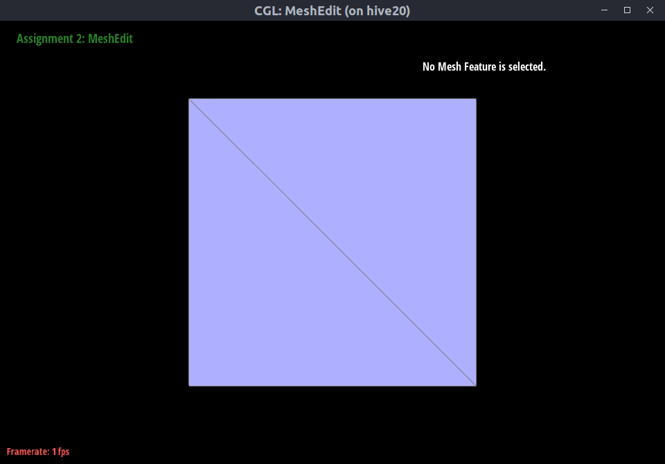
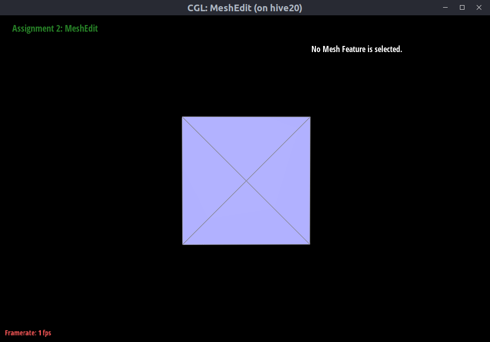
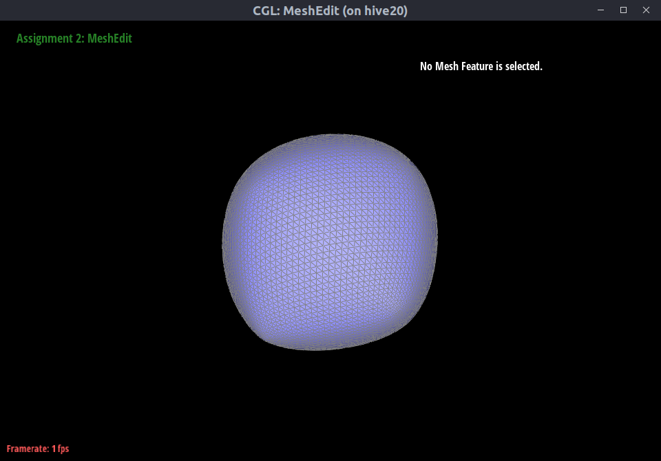
Load dae/cube.dae. Perform several iterations of loop subdivision on the cube. Notice that the cube becomes slightly asymmetric after repeated subdivisions. Can you pre-process the cube with edge flips and splits so that the cube subdivides symmetrically? Document these effects and explain why they occur. Also explain how your pre-processing helps alleviate the effects.
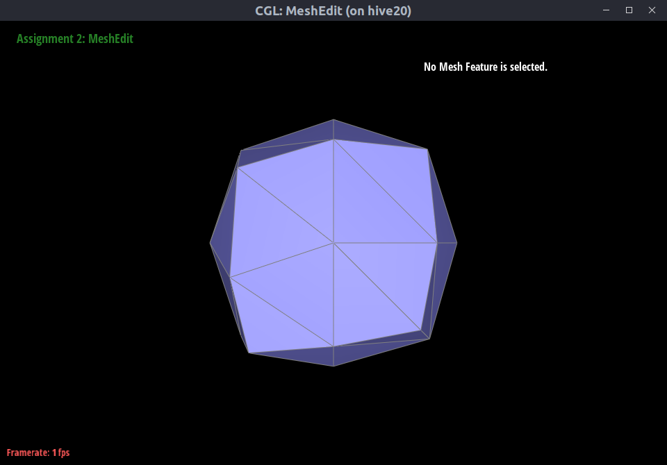
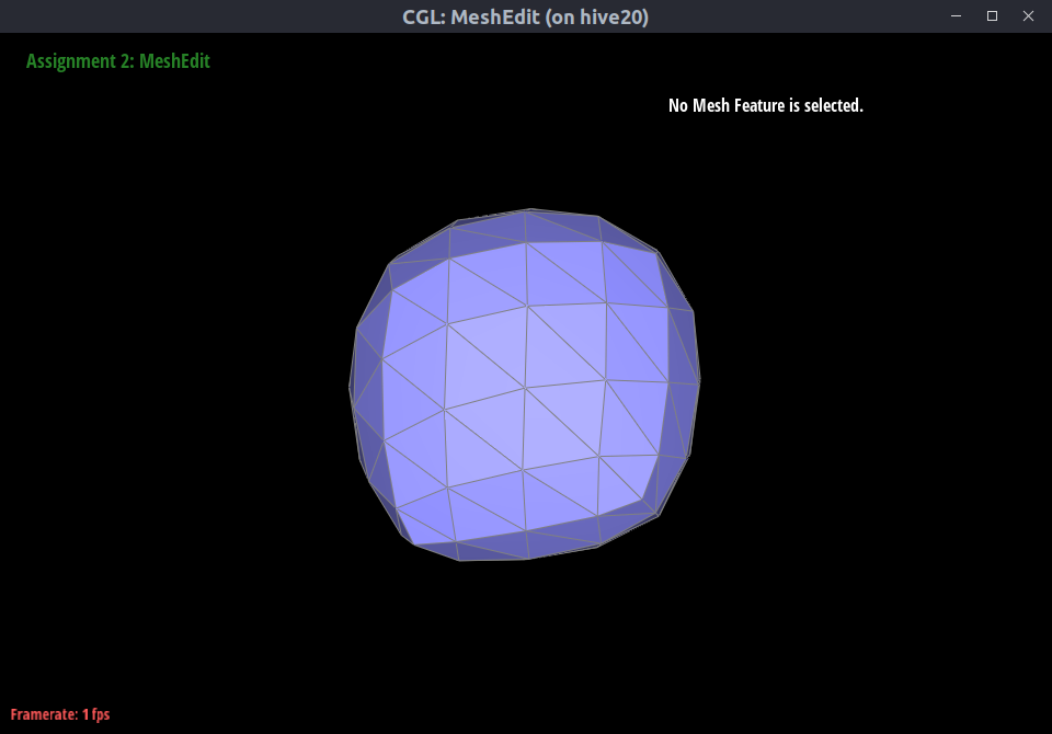
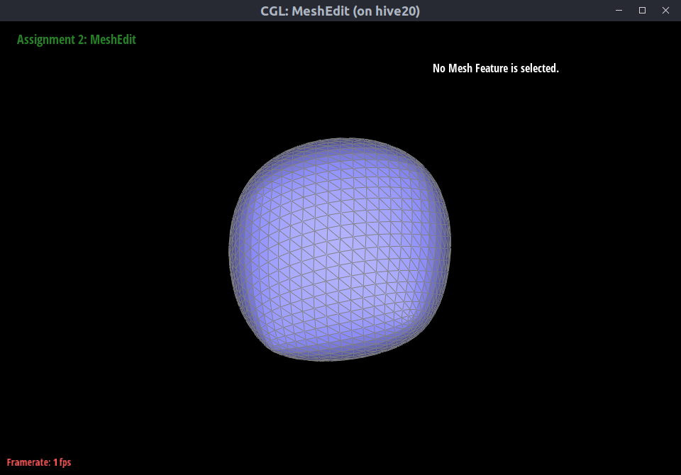
If we don’t pre-process the cube, the subdivisions look like this. As we can see, the mesh gradually becomes asymmetric with respect to the horizontal and vertical axis of the plane of the front-facing cube surface.

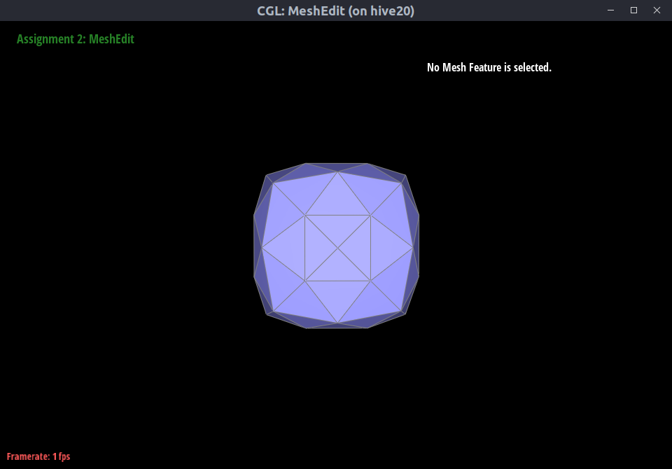
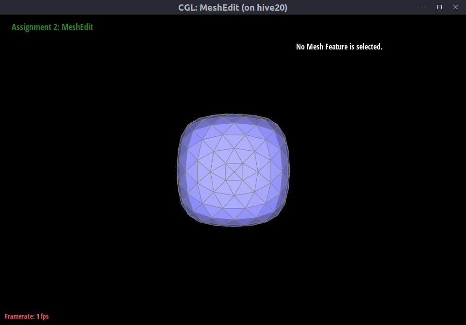
Looking at the topology of the cube, we can observe that the diagonal edge on each face is asymmetric, which is the reason why the above effect occurs. To make the edges symmetric, we can split each of them once to obtain a cross. As we observe below, the result of Loop subdivision is now symmetric with respect to the horizontal and vertical axis of the plane of the front-facing cube surface.