Rasterizer

This is a CS184 Project. For graders, if you are looking for a list of rubric items and their locations within this post, please scroll to the bottom of the page. For everyone else, please read on.

Overview

Rasterization is a method of taking in mathematical descriptions of a scene and turning it into pixel values that we can display on a screen. As a simple example, imagine if we have a triangle defined by three vertices: $(0, 0), (5, 0), (5, 5)$. Since most of our screens consist of a grid of pixels, then in order to display this triangle, we will need to fill in the framebuffer at each point on the grid with a color. This process is called rasterization. Although the objects being rasterized are most commonly triangles, rasterization can be applied to other shapes as well.

In this project, we implement a CPU rasterizer that has multiple mipmap modes, multiple pixel sampling modes, multiple levels of supersampling, the ability to render texture, and the ability to render affine transforms.

Rasterizing single-colored triangles

In this part, we implement a simple CPU rasterizer that draws a triangle with a single color.

void RasterizerImp::rasterize_triangle(float x0, float y0,
                                       float x1, float y1,
                                       float x2, float y2,
                                       Color color);

The first step is to calculate the bounding box of the triangle. After all, we wouldn’t want to loop through the whole pixel buffer if our triangle only occupies a small portion of it. This is achieved by taking the minimum and maximum of the coordinates to obtain two diagonal corners of the bounding box.

The second step is to loop through each sample point in our bounding box, checking whether they land within the triangle. To do this, we’ll use some maths.
We will first assume the winding order of the triangle to be counter-clockwise. That is, the vertices $(x0, y0), (x1, y1), (x2, y2)$ enclose the triangle in a counter-clockwise order. In the end, we’ll generalize our result to any arbitrary winding order.

Now, rotate the edges vectors of this triangle counter-clockwise by 90 degrees. We obtain three normal (i.e. perpendicular) vectors.

Notice that all of the newly rotated vectors now point inwards. Observe that if a point is ‘on the same side’ of the edge as the normal vector for every edge, then this point must be inside the triangle. To see how this could be tested, let’s focus on a single edge.

Let $P=(x,y)$ be an arbitrary sample point, $N$ be a normal vector to the line defined by $P_0$ and $P_1$, $V = P - P_0$. We want to figure out if $N$ and $V$ are ‘on the same side’ of the line as each other. From the diagram, we can see that $V \cdot N = |V||N|cos\theta > 0 \iff$ $V$ and $N$ are on the same side. Now we just need to calculate $N \cdot V$ for each edge, checking whether they are all positive to determine whether a point is in a triangle!

Now if we reverse the winding order, the rotated vectors will all turn outwards. Can we still use a similar method to determine whether a point lands in a triangle? Yes! Instead of testing whether all of $V \cdot N$ is $>0$, we test if all of them are $<0$.

We now have a general algorithm for testing if a point lands in a triangle, regardless of winding order. Observe that in either winding order, if a point does not land inside the triangle, exactly one of the $V \cdot N$ values will have a different sign compared to the other two. However, if a point does land inside the triangle, $V \cdot N$ of all edges will share the same sign.

In the actual implementation, we first generate functions $V \cdot N = L(P)$ for all three edges. Then we loop through the sample points in the bounding box, evaluating the three $L(P)$s at that point, and comparing their sign.

$L(P) = V \cdot N = (P - P_0) \cdot N = (P - P_0) \cdot M_{rot 90}(P_1 - P_0)$

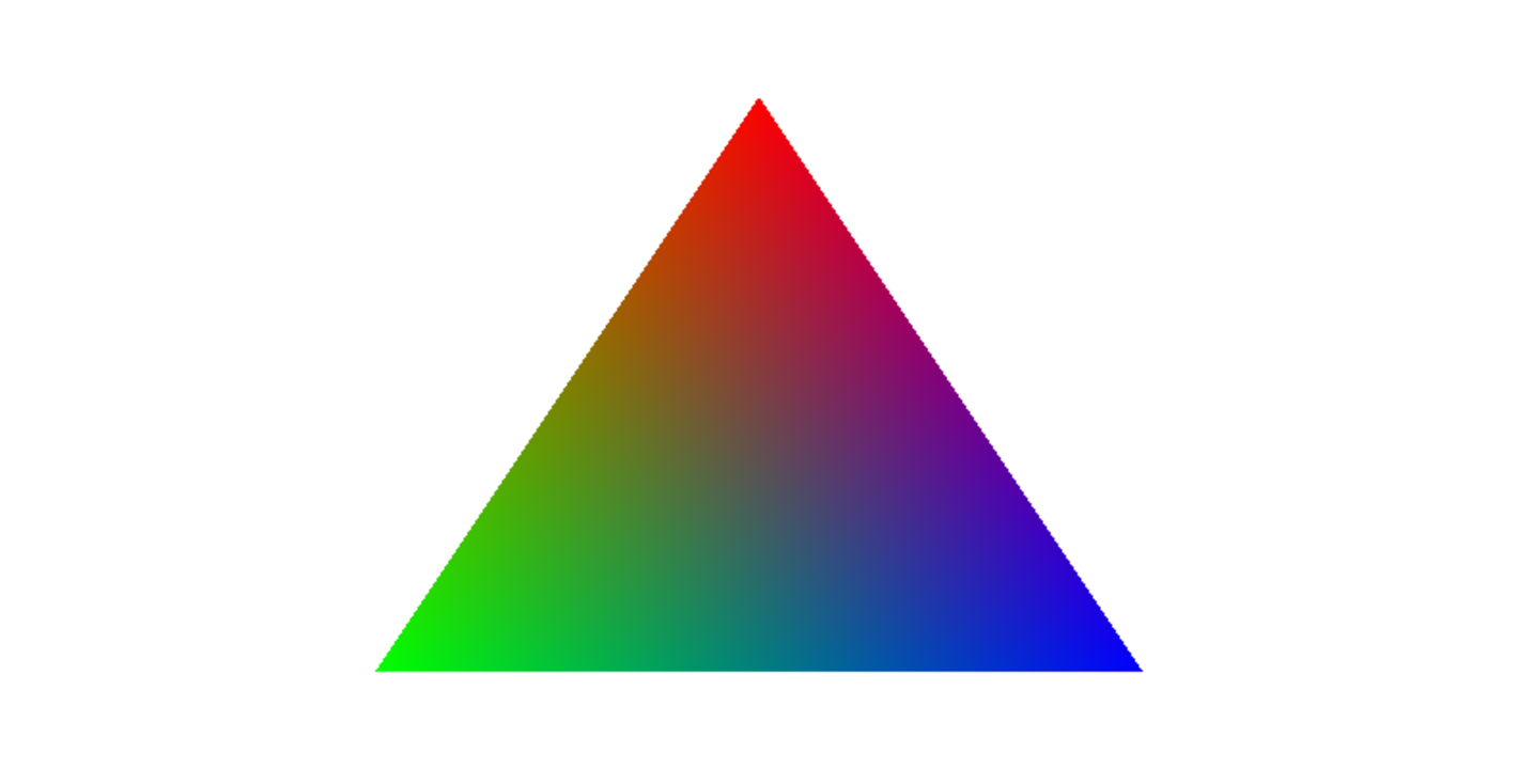
Barycentric Coordinates

Now that we have triangles on the screen, it’s time to give it some color - or textures. In order to do that, we need to figure out at each sample where the sample lands on the triangle (so we can apply the texture accordingly). Barycentric coordinates are a widely adopted way to do this.

In essence, barycentric coordinates are simply a set of numbers that describe a linear combination of vertices of a given triangle.
For $\triangle ABC$, if $P = (\alpha, \beta, \gamma)$, where $\alpha + \beta + \gamma = 1$, and $A$, $B$, $C$ each has an associated value, then

$P = \alpha A + \beta B + \gamma C$

For instance, we can use it to describe location inside a triangle. The midpoint between vertices $B$ and $C$ can be described in barycentric coordinates as $(0, 0.5, 0.5)$.

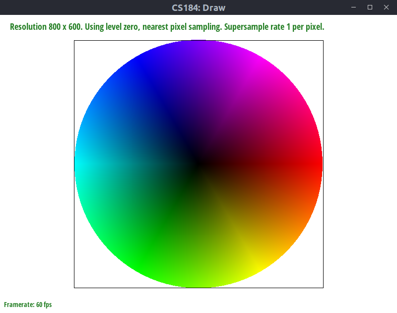
Representing location with barycentric coordinates is certainly useful, but its power lies in its ability to naturally map a location on a triangle to other data. For example, we can use it to map color. If we define the three vertices of a triangle to be of the color red, blue, and green respectively, then for any point $P$ in the triangle, we can map its barycentric coordinates to a color defined as $C(P) = \alpha A + \beta B + \gamma C$. The result is a triangle with smooth color transitions:

Rubric

If you are a project grader, this section is for you. For everyone else, the following section may be slightly cryptic.

• See Overview

Task 1

• Walk through how you rasterize triangles in your own words.
  See Rasterizing single-colored triangles
• Explain how your algorithm is no worse than one that checks each sample within the bounding box of the triangle.
  As explained in the above link, my code literally loops through each sample within the bounding box of the triangle, so it is no worse than one that checks each sample within the bounding box of the triangle.
• Show a png screenshot of basic/test4.svg with the default viewing parameters and with the pixel inspector centered on an interesting part of the scene.
  
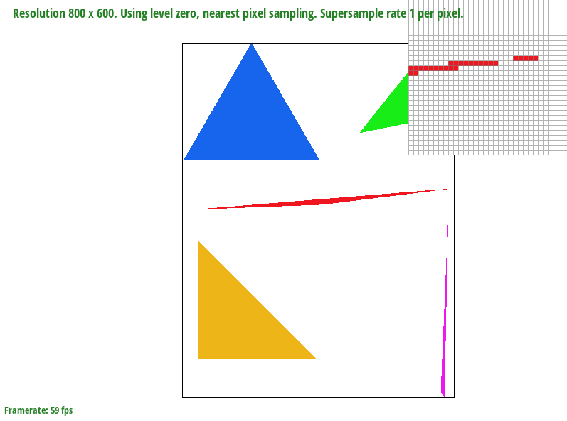
  This image is interesting because it shows the aliasing artifacts of the red triangle.

Task 2

• Walk through your supersampling algorithm and data structures. Why is supersampling useful? What modifications did you make to the rasterization pipeline in the process? Explain how you used supersampling to antialias your triangles.
  My supersampling algorithm still loops through the bounding box, pixel by pixel. However, within each pixel I calculate sample_x and sample_y by incrementing delta = 1.0f / sqrt(sample_rate) amount in either the x-direction or the y-direction. The result is a grid of subsamples shown in the spec. Every time I obtain a value, I store it into a vector of Color objects called supersample_buffer, which has a size of width * height * sample_rate.
  supersampling is useful because by taking more samples around a given pixel and averaging those samples, we are essentially applying a 1-pixel-sized box filter at each pixel, which helps to filter out high frequencies in the image and thus reduce aliasing.
  I took a minimalistic approach to modifying the pipeline. Aside from the changes mentioned above in rasterize_triangle, I also made some small changes in other places. In resolve_to_framebuffer, I looped through each pixel and averaged the subsamples of that pixel before putting them into the image buffer. In order to render lines and dots correctly, I changed rasterize_point to write to the super sample buffer instead of the image buffer, so that its results won’t get overwritten by resolve_to_framebuffer. Since rasterize_line simply calls rasterize_point, that takes care of lines as well.

• Show png screenshots of basic/test4.svg with the default viewing parameters and sample rates 1, 4, and 16 to compare them side-by-side. Position the pixel inspector over an area that showcases the effect dramatically; for example, a very skinny triangle corner. Explain why these results are observed.
  
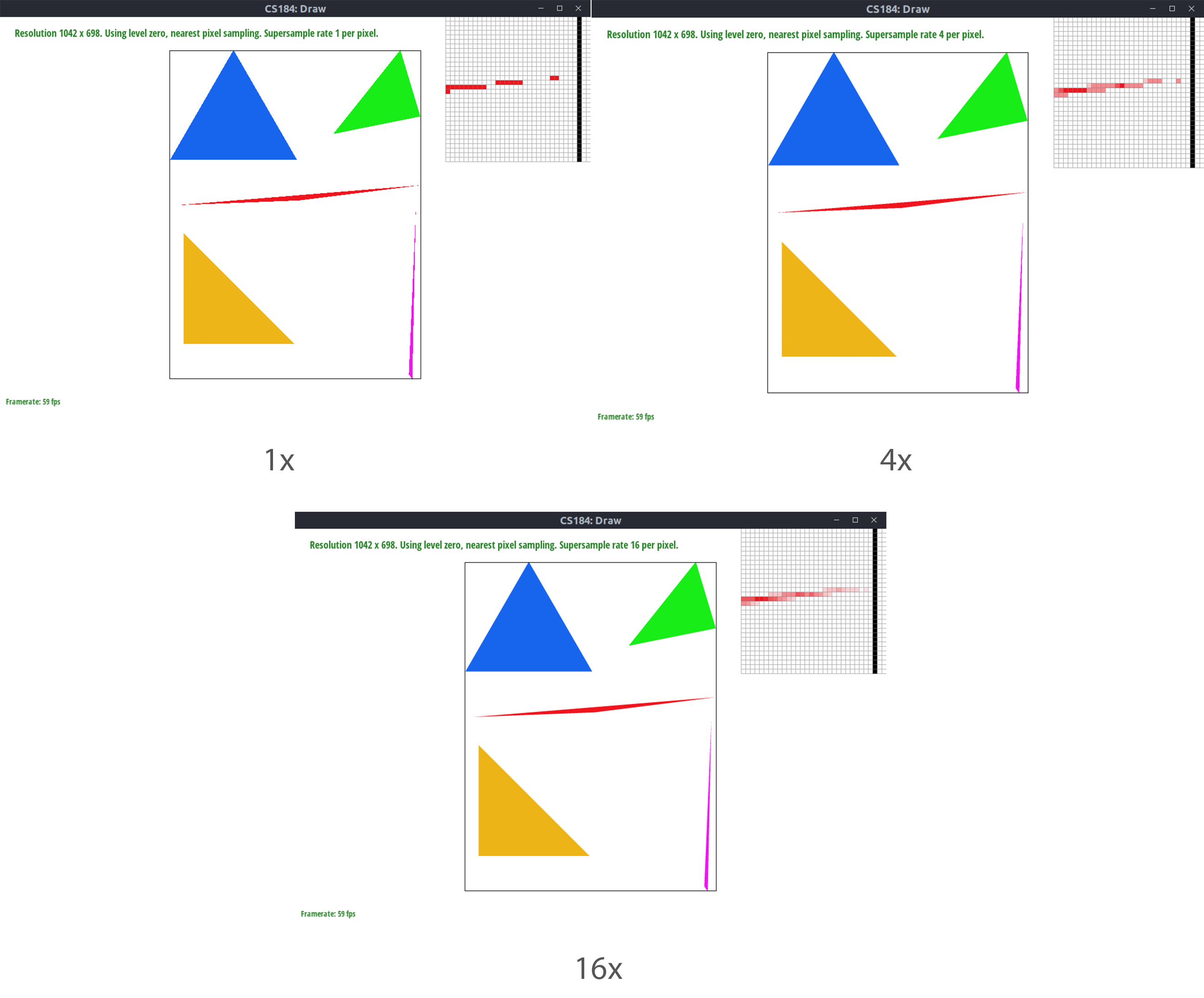
  These results are observed because having a higher sampling rate means our pre-filter approximates the box filter better, thus we get less aliasing. Shown on the image, this means as we increase the sampling rate, the smoother the edge of the triangle becomes.

Task 3

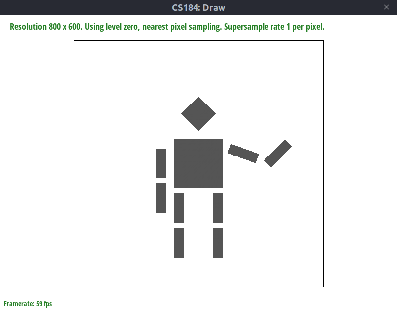
• Create an updated version of svg/transforms/robot.svg with cubeman doing something more interesting, like waving or running. Feel free to change his colors or proportions to suit your creativity. Save your svg file as my_robot.svg in your docs/ directory and show a png screenshot of your rendered drawing in your write-up. Explain what you were trying to do with cubeman in words.
  I decided to make the robot wave. I first rotated the outer part of the right arm by 45 degrees, then the inner part of the right arm by 20 degrees. This creates a waving gesture, but the position is off, so applied an additional translation. For the left arm, I rotated the entire object by 90 degrees, then applied another translation to move it by the robot’s body.
  

Task 4

• Explain barycentric coordinates in your own words and use an image to aid you in your explanation. One idea is to use a svg file that plots a single triangle with one red, one green, and one blue vertex, which should produce a smoothly blended color triangle.
  See Barycentric Coordinates

• Show a png screenshot of svg/basic/test7.svg with default viewing parameters and sample rate 1. If you make any additional images with color gradients, include them.
  

Task 5

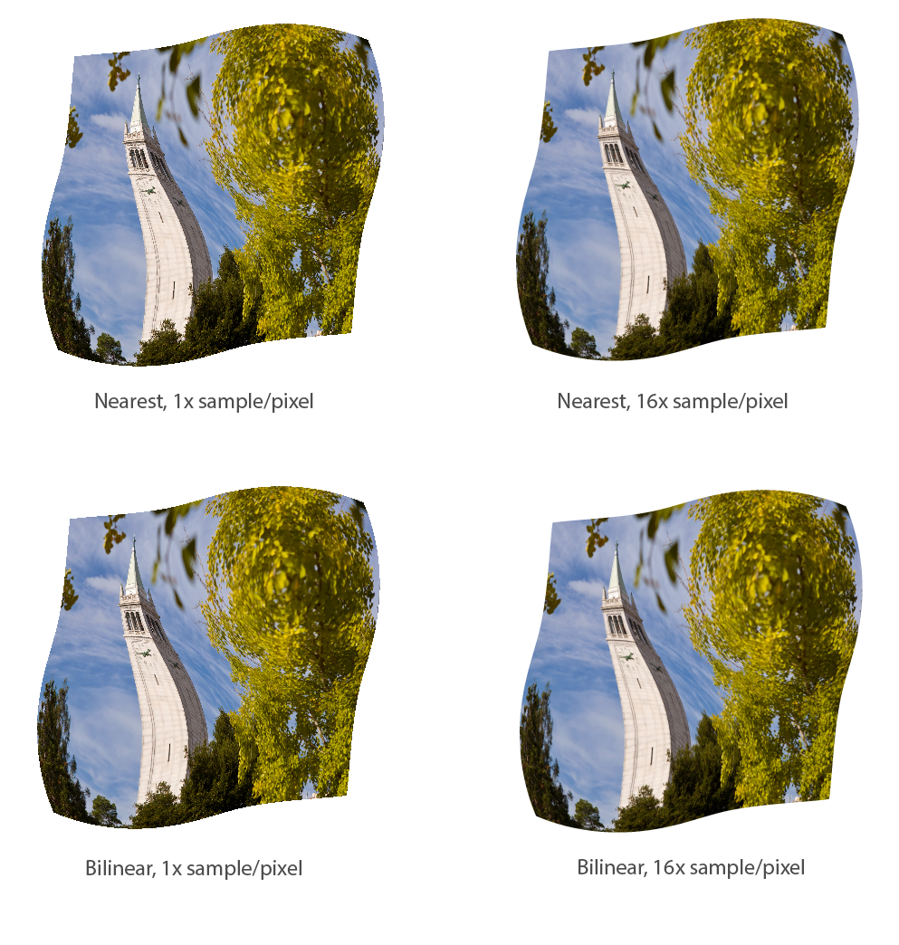
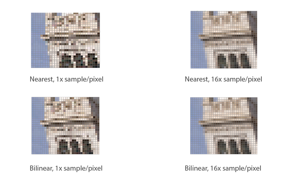
• Explain pixel sampling in your own words and describe how you implemented it to perform texture mapping. Briefly discuss the two different pixel sampling methods, nearest and bilinear.
  Pixel sampling is the process of determining the color of a pixel by sampling the underlying texture of a surface. Nearest neighbor is the simplest method: we first determine where a pixel lands in the texture coordinate $(u,v)$ by barycentric coordinates, and then use the texture pixel that’s closest to that coordinate. Bilinear sampling takes the four nearest texture pixels in texture space and weights them. The closer the coordinate to a given pixel, the more weight it gets. A good diagram illustrating bilinear sampling could be found here. Because bilinear sampling provides a continuous mapping of texture coordinates to colors, it appears more smooth than nearest neighbor.
  As for the actual implementation, I wrote two functions sample_nearest and sample_bilinear. Both take a (u,v) position and a mipmap level. sample_nearest multiplies that $(u,v)$ with the dimension of the texture, rounds it, and returns the color stored at that position. sample_bilinear also multiplies $(u,v)$ with the dimension of the texture, but instead of rounding it, it takes both the ceiling and floor of the coordinates to obtain the four nearest texture pixels available. Then, it performs a weighted average using the relative position of the sample point to the texture pixels, and returns the final color.

• Check out the svg files in the svg/texmap/ directory. Use the pixel inspector to find a good example of where bilinear sampling clearly defeats nearest sampling. Show and compare four png screenshots using nearest sampling at 1 sample per pixel, nearest sampling at 16 samples per pixel, bilinear sampling at 1 sample per pixel, and bilinear sampling at 16 samples per pixel.
  
  

• Comment on the relative differences. Discuss when there will be a large difference between the two methods and why.
  The difference between nearest and bilinear could be best observed with the set of 1x sample/pixel images. The lines in the image resulted from bilinear sampling are clearly smoother and contain less noise compared to those from nearest neighbor. The difference exists because this portion of the image contains many fast changing (i.e. high frequency) details, so prefiltering with bilinear interpolation helps to smooth these details out. Similar differences can be observed in the 16 samples/pixel pair, though they are less pronounced, because supersampling also helps to filter out the high frequency details.

Task 6

• Explain level sampling in your own words and describe how you implemented it for texture mapping.

When we map a texture from texture space to screen space, we may face two difficulties:

1. The texture is too small, so it appears stretched and blocky
2. The texture is too large, so pixels on the screen are not enough to sample it, leading to aliasing.

Level sampling partially solves these problems by storing different levels of low-pass filtered and down-sampled textures for any given image. Depending on whether the underlying surface is close or far away, different versions of those images are used. Our rasterizer implements three modes:

1. level zero: only use the full resolution texture
2. nearest: find the level that most closely matches the screen resolution and use that level’s texture.
3. bilinear: calculate the ideal level that matches the screen resolution (note this will be a floating point number). Then interpolate two levels that are closest to this ideal level. For example, if we know are screen resolution corresponds to level 3.2, we would interpolate between levels 3 and level 4.

Level $D$ can be calculated using the equation

$D = log_2 L$

$L = max(\sqrt{\frac{du}{dx}^2 + \frac{dv}{dx}^2}, \sqrt{\frac{du}{dy}^2 + \frac{dv}{dy}^2})$

In plain words, this equation calculates the maximum texture space coordinate change that happens corresponding to $1$ unit of coordinate change in screen space on either the x or the y direction. If the change is more rapid, level $D$ is also higher.

In the implementation, rasterize_textured_triangle populates a SampleParams struct that contains the location of the sample point, the derivatives used in the above implementation, and the sampling mode (0, nearest, or bilinear). This struct is then passed to sample, which calculates the level from the given derivatives and either calls sample_nearest or sample_bilinaer depending on the mode.

• You can now adjust choosing between pixel sampling and level sampling as well as adjust the number of samples per pixel. Analyze the tradeoffs between speed, memory usage, and antialiasing power between the various techniques at different zoom levels.

In terms of speed, 1 pixel per sample is the fastest compared to sampling more than once. Nearest neighbor is faster than bilinear interpolation in pixel sampling. In level sampling, nearest and level-0 are similar in speed because the only extra calculation that nearest has is level calculation. Bilinear is slower than both, because it essentially weights the two nearest level sampling results.

In terms of memory usage, the amount of memory required scales linearly with the number of samples per pixel because a bigger buffer is required (in my implementation). The amount of memory required is roughly the same between bilinear pixel sampling and nearest pixel sampling, because we are only averaging on each pixel and not storing much extra information. The amount of memory required for bilinear, nearest, and level-0 are also similar, for the same reason. However, note that in order to store more levels for nearest and bilinear to work, we need roughly $4/3$ times the memory required for storing only level 0.

In terms of antialiasing power, the combination of 16 samples per pixel, bilinear level sampling, and bilinear pixel sampling is the best. Antialiasing power decreases in the order of 16x supersampling -> 9x -> 1x, bilinear level sampling -> nearest level sampling -> level 0, bilinear pixel sampling -> nearest pixel sampling. This is true in general, though if we are on the boundary of a particular level throughout the image, then bilinear level sampling performs the same as nearest level sampling because we are only sampling one level either way.

• Show at least one example (using a png file you find yourself) comparing all four combinations of one of L_ZERO and L_NEAREST with one of P_NEAREST and P_LINEAR at a zoomed out viewpoint.
  

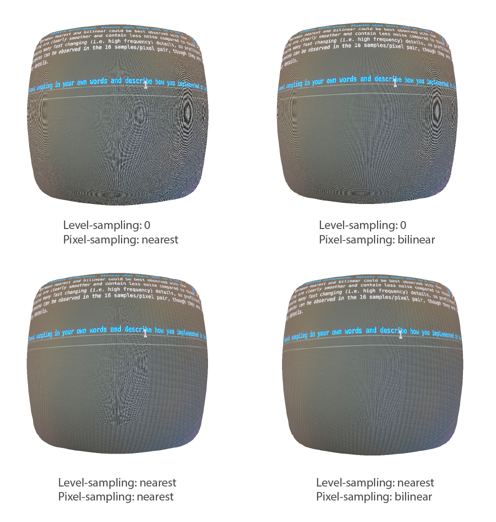
Here, we can see that level 0, nearest performs the worst and level nearest, p linear performs the best.